2 Basic single cell pipeline
The steps below encompass the standard pre-processing workflow for scRNA-seq data.
- Filter out low quality cells: undersequenced cells, debris (broken cells or floating pieces of RNA) and multiplets (several cells in one droplets)
- Normalize the UMI expression to reduce the sequencing biais (some cells are less sequenced than others).
2.1 Remove “low quality” cells
The are a few metrics commonly used to filter out low quality cells :
- the number of unique genes detected in each cell
- cells with low gene count : helps to remove empty droplets, debris and undersequenced cells.
- cells with high gene count : these cells are more likely to be cell doublets or multiplets. The number of multiplets expected in your sample is directly correlated with the number of cells you loaded in 10X. The more cells you loaded, the higher the chance is to have 2 or more cells in one droplet.
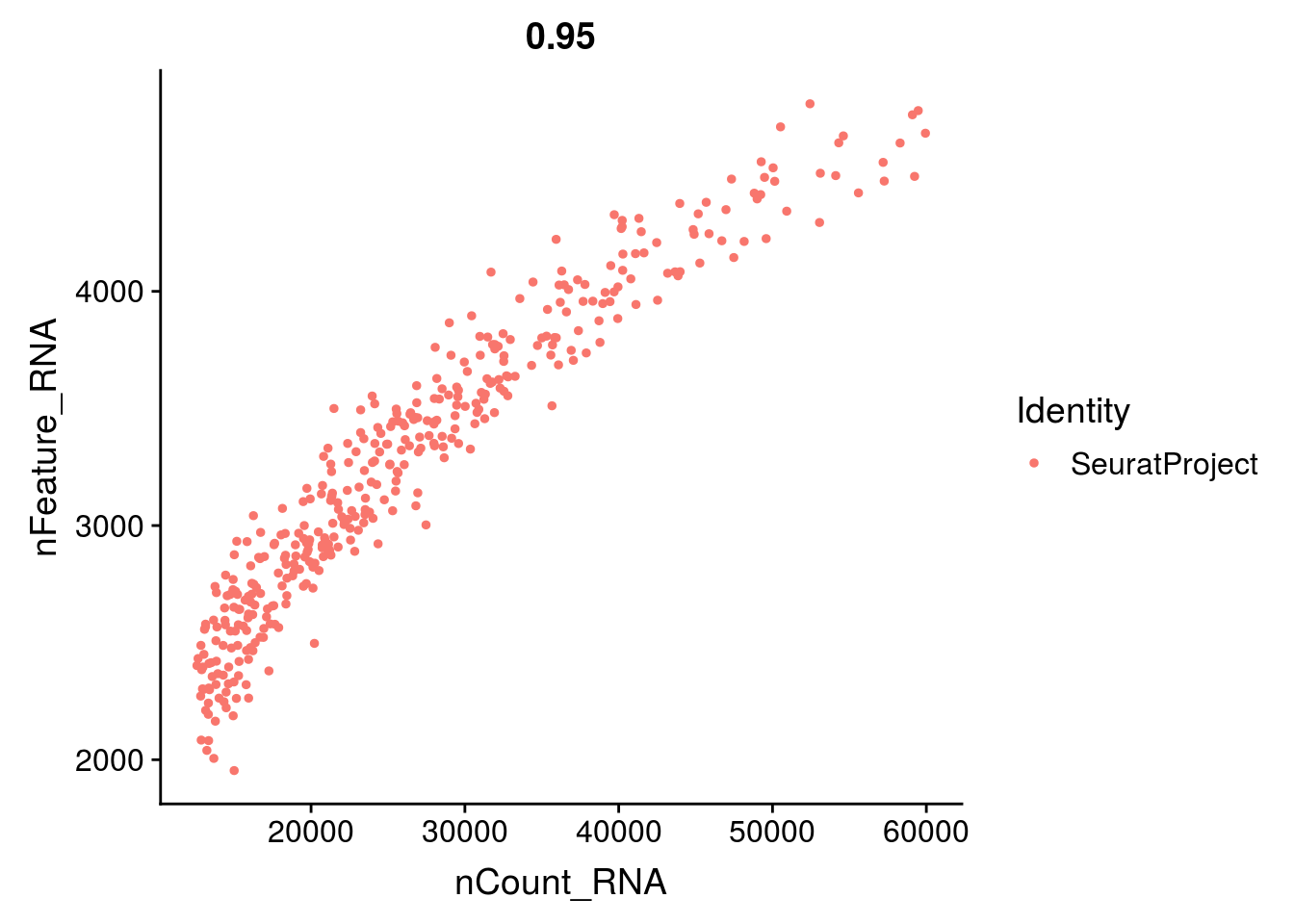
- the total number of UMI detected within a cell
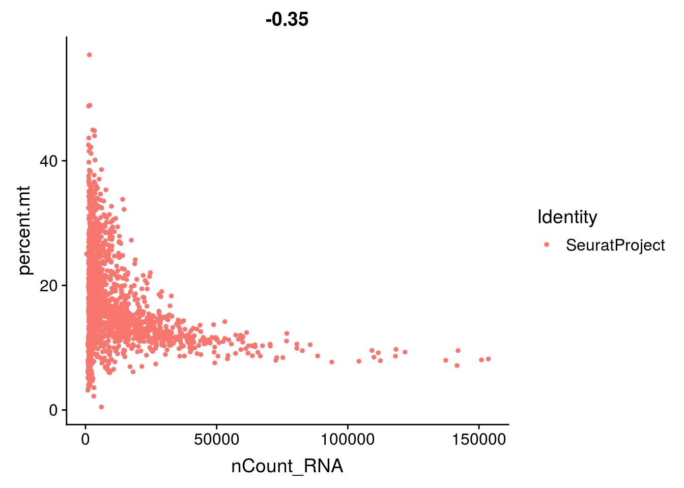
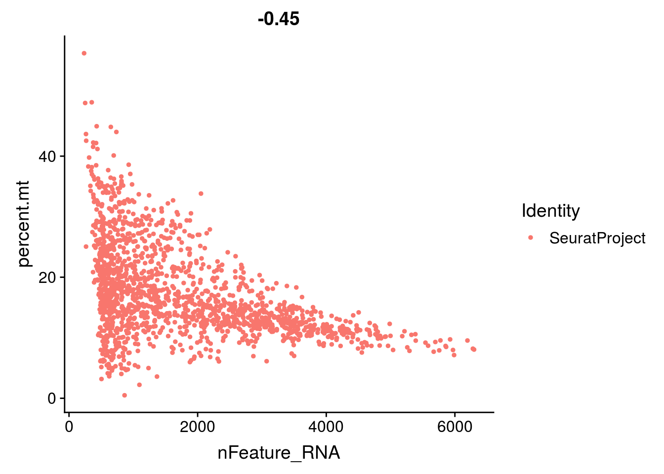
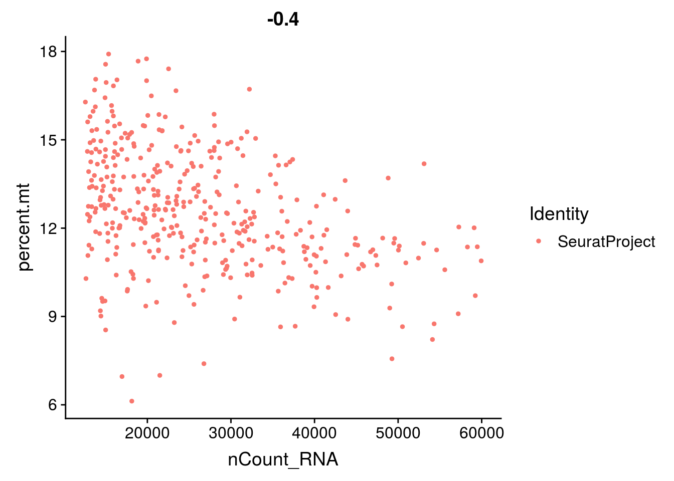
- the total number of UMI and the number of genes are highly correlated. Looking at the scatter plot between these two variables helps you detect atypical cells.
- the percentage of reads that map to the mitochondrial genome
- low-quality / dying cells often exhibit extensive mitochondrial contamination
Seurat allows you to easily explore these QC (quality control) metrics and filter out cells.
2.1.1 Number of genes detected per cell
hist(mydata$nFeature_RNA,
     breaks = 200,
     xlab = "n genes",
     main = "Number of genes detected / cell"
     )
#add a vertical line to your plot to help you choose a threshold
abline(v = 6000 , col = "red")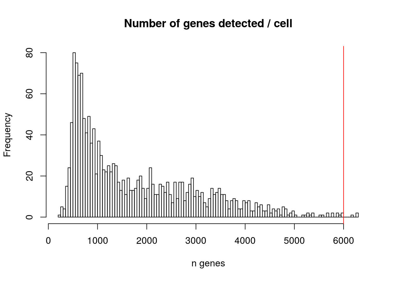
##     0%    25%    50%    75%   100%
##  235.0  705.0 1308.0 2588.5 6298.0
2.1.2 Number of UMIs per cell
hist(mydata$nCount_RNA,
     breaks = 50,
     xlab = "Total UMIs per cell",
     main = "Number of UMI / cell"
     )
abline(v = 150000 , col = "red") 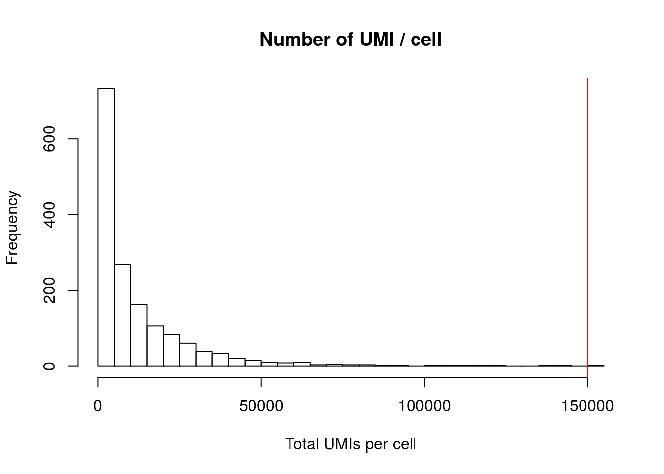

Your aim while looking at these graphs is to define the thresholds/cutoffs that you will apply to filter cells out. To do so, try to identify the cells that behave differently from the main population.
2.1.3 Percentage of mitochondrial genes
To calculate the percentage of mitochondrial genes expressed in a cell, you must first provide a list of mitochondrial genes. In the paper, the authors did not provide their list. As a quick replacement, we will consider that mitochondrial genes are all the genes that starts with the pattern mt:. For a more refine analysis, you can use flybase or another source and carefully identify mitochondrial genes.
We then use the PercentageFeatureSet function, which calculates the percentage of counts originating from a set of features.
mydata[["percent.mt"]] <- PercentageFeatureSet(mydata, pattern = "^mt:")

# Alternative : if you have a list of mitochondrial genes
#list = c("mTerf3","Mtpalpha" ,"mTTF")
#mydata[["percent.mt2"]] <- PercentageFeatureSet(mydata, features=list_mito )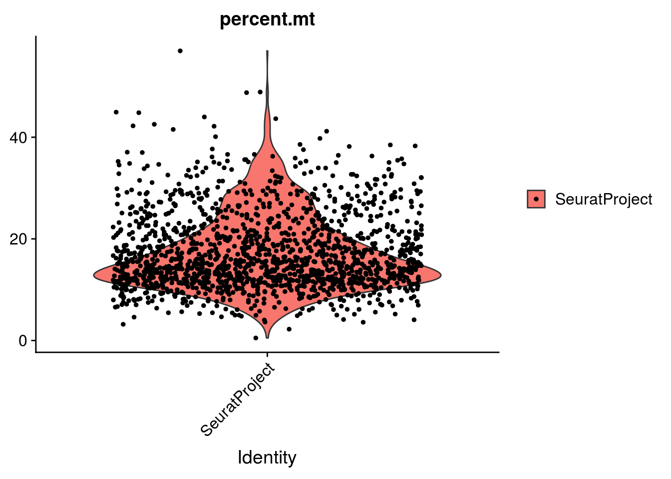
2.1.4 Group exercise on filtering
One of the most difficult parts of single cells pre-processing is to decide the thresholds to define low and high quality cells. From the various graphs above, decide the levels for low high quality cells dependent on the number of genes expressed per cell, the total UMIs per cell and the percentage of mitochonrial genes.
Discuss your cutoff as a group.
# DEFINE THE CUTOFF VALUES FOR EACH VARIABLE AND VISUALIZE THE RESULTS.
minGene    =
maxGene    =
minUMI     =
maxUMI     =
maxpct_mt  =
# the function "subset" helps you to filter the cells
# we create a new seurat object containing the filtred cells
mydata_filtrd <- subset(mydata, subset = nFeature_RNA > minGene &
nFeature_RNA < maxGene &
nCount_RNA > minUMI &
nCount_RNA < maxUMI &
percent.mt < maxpct_mt)
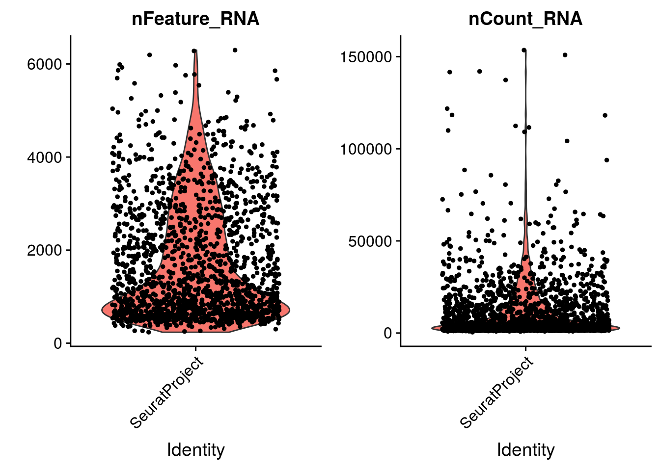
VlnPlot(mydata_filtrd, features = c("nFeature_RNA", "nCount_RNA", "percent.mt"), ncol = 3)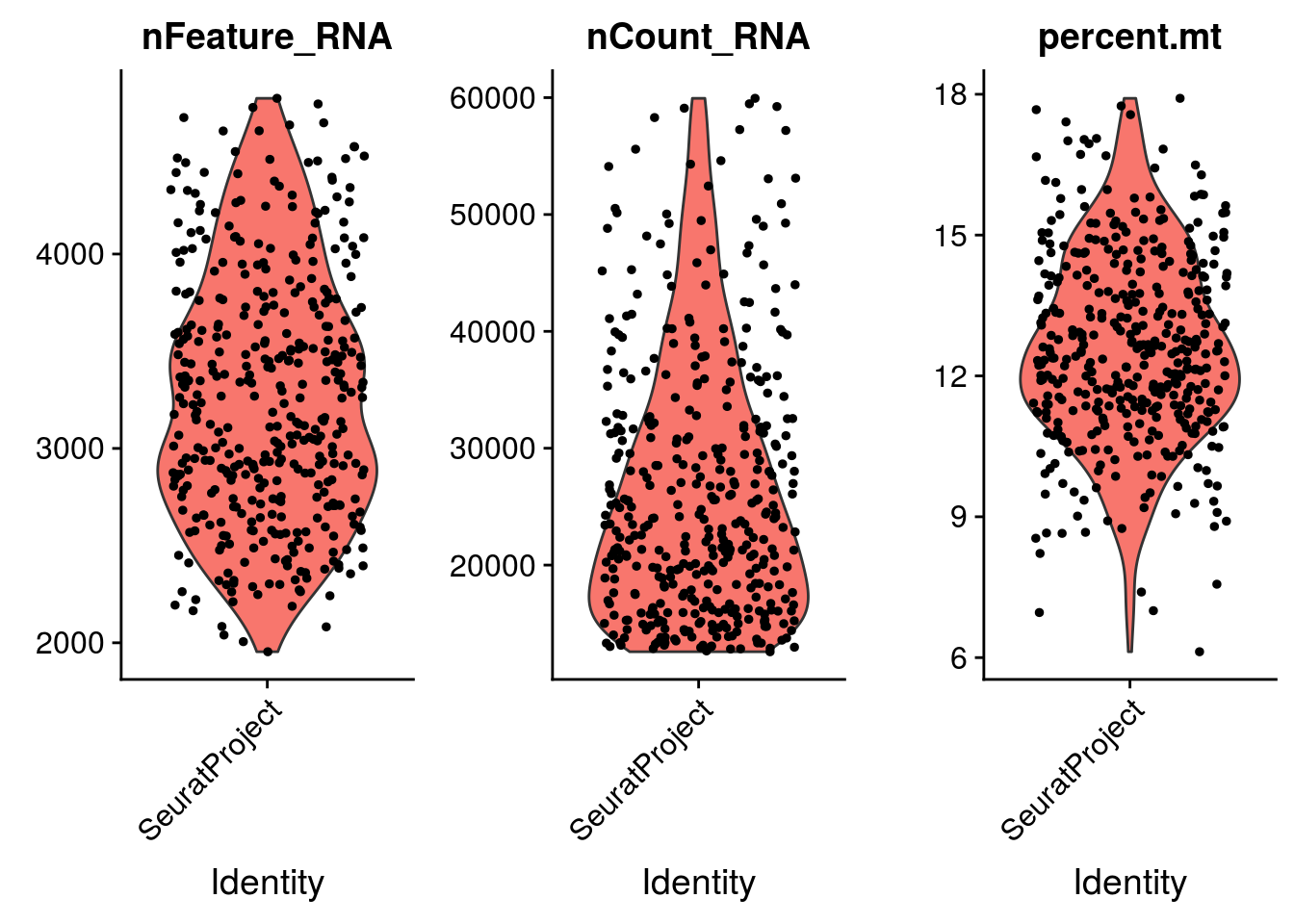
2.2 Normalize the expression in cells
As we noticed in the previous graphes, the cells do not have the same number of total UMIs. This may be due biological differences (some cells express less RNA than other) but is likely to be the result of cell-specific sequencing biais (some cells have been less sequenced than other). The normalization step aims to correct for this bias.
We are going to apply a global scaling method, which supposes that all cells have about the same RNA content. The LogNormalize method normalizes the expression measurements for each cell by the total expression, multiplies this by a scale factor (here the median total UMI per cell), and log-transforms the result.
mydata_filtrd <- NormalizeData(mydata_filtrd,
                               normalization.method = "LogNormalize",
                               scale.factor = median(mydata_filtrd$nCount_RNA))
The resulting data is stored in the data slot.
Once you have pre-processed your data, you are ready for further analyses (e.g. identify sub-population of cells, pseudo-time analyses).